1. Why Token Count Matters More Than You Think

Every time your application calls a large language model, you pay per token — for every word of context you send, and every word the model generates back. In production, this compounds fast.

Consider a simple customer support bot running on Claude 3.5 Sonnet via Amazon Bedrock, answering 1,000 queries per day. If each query injects 2,000 tokens of retrieved context, that's 2 million context tokens daily — costing $6/day just for input, or $180/month. Scale to 10,000 queries and you're looking at $1,800/month on input tokens alone, before a single output token is counted.

The good news: the architecture of how you retrieve and inject context has a dramatic effect on this number. Three distinct patterns have emerged in production AI systems:

These numbers come from running 20 standardised queries across all three implementations on AWS Bedrock with anthropic.claude-sonnet-4-6 as the inference model. Let me walk you through how each works, how to build it, and critically — when to use which.

2. The Three Retrieval Patterns Explained

Retrieval-Augmented Generation (RAG)

RAG is the dominant pattern for grounding LLMs in external knowledge. Documents are split into chunks, embedded into vectors using a text embedding model (Amazon Titan Embeddings V2 in our case), and stored in a vector index. At query time, the user's question is also embedded and the top-k most semantically similar chunks are retrieved and injected into the prompt.

RAG's primary strength is flexibility: it handles large, dynamic knowledge bases that change frequently, and it scales to millions of documents without hitting context window limits. Its weakness is cost — every query pays the full price for embedding lookup plus context injection.

Cache-Augmented Generation (CAG)

CAG takes a radically different approach: instead of retrieving relevant chunks at query time, it loads the entire knowledge base into the system prompt and marks it with cache_control: {"type": "ephemeral"}. Amazon Bedrock caches this prompt prefix server-side. The first query writes to cache at +25% cost; every subsequent query reads from cache at −90% cost.

The result: after warmup, the model already has all the context it could ever need, and you pay almost nothing for re-reading it. This is transformative for static or slowly-changing knowledge bases — FAQ documents, product catalogues, policy handbooks, API reference guides.

Knowledge-Augmented Generation (KAG)

KAG uses a knowledge graph (Amazon Neptune) as the retrieval source. Instead of unstructured text chunks, the knowledge base is stored as a network of entities (nodes) and relationships (edges). At query time, key entities are extracted from the question, Neptune is traversed to find the relevant subgraph, and the resulting facts are serialised into a compact, structured context.

Because graph facts are concise ("Bedrock → supports → PromptCaching → reduces → InputTokenCost"), KAG produces the smallest context of the three methods — typically 200–600 tokens — without sacrificing answer precision for in-graph questions.

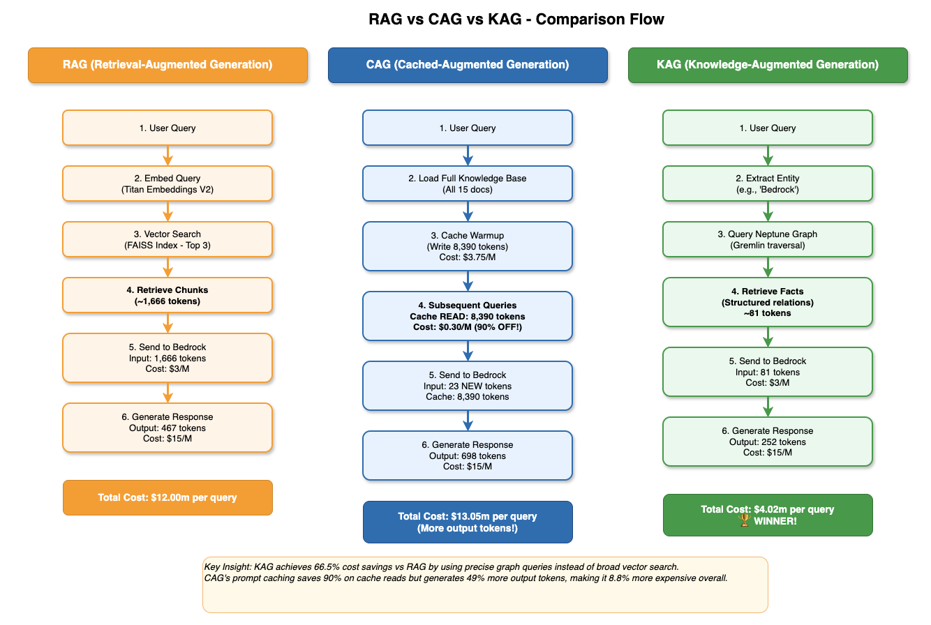
Figure 1 — Side-by-side comparison of all three retrieval flows. RAG embeds and retrieves chunks at query time ($12.00m/query). CAG reads from Bedrock's server-side prompt cache after warmup ($13.05m with more output, but 90% cheaper on cache reads). KAG traverses Neptune's graph and wins on cost at $4.02m/query.

Reading Figure 1 left to right tells the whole story. RAG (orange) runs 6 steps on every single query — embed the question, search FAISS, retrieve 1,666 tokens of chunks, send to Bedrock — and pays the full $3/1M input rate each time. There is no amortisation: query #1,000 costs exactly the same as query #1. CAG (blue) front-loads the work: the cache warmup step writes 8,390 tokens once at $3.75/1M, then every subsequent query reads those same tokens from the cache for $0.30/1M — a 10× discount. The catch is that CAG generates more output tokens (698 vs 467 for RAG), because having the full knowledge base in context tends to produce longer, more detailed answers. KAG (green) skips embedding entirely. Two steps — entity extraction and Neptune graph traversal — produce just 81 structured facts, totalling around 387 tokens. That extreme context precision is why KAG wins on cost despite paying the same $3/1M input rate as RAG.

3. AWS Architecture & Infrastructure

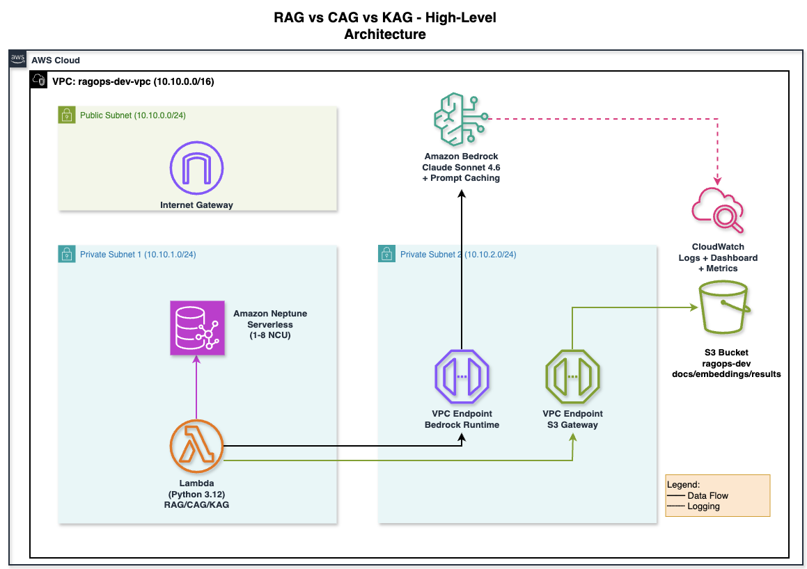
Figure 2 — High-level AWS architecture for the RagOps project. All three pipelines run inside a private VPC (10.10.0.0/16). Lambda (Python 3.12) connects to Amazon Bedrock via a VPC Interface Endpoint and to S3 via a Gateway Endpoint — no NAT Gateway needed. Amazon Neptune Serverless (1–8 NCU) lives in a separate private subnet. CloudWatch captures invocation logs, token metrics, and latency.

The architecture is deliberately designed so that no traffic leaves the AWS network. The Lambda function (bottom-left) lives in a private subnet with no route to the internet. When it calls Bedrock, the request goes through the VPC Interface Endpoint for bedrock-runtime — a private network path that stays entirely within AWS. S3 access goes through a Gateway Endpoint, which is free and routes through AWS's internal network. The only reason there is a public subnet and Internet Gateway in the diagram is to provide outbound internet for future tooling (e.g., downloading Python packages during Lambda deployment) — the core pipelines never use it. Neptune lives in its own private subnet (10.10.1.0/24), reachable only from the application subnet via the security group rules. CloudWatch receives invocation logs via the Bedrock logging role — shown as the dashed line — so you get token metrics without any additional instrumentation in your code.

All three pipelines share a common AWS foundation, provisioned with Terraform:

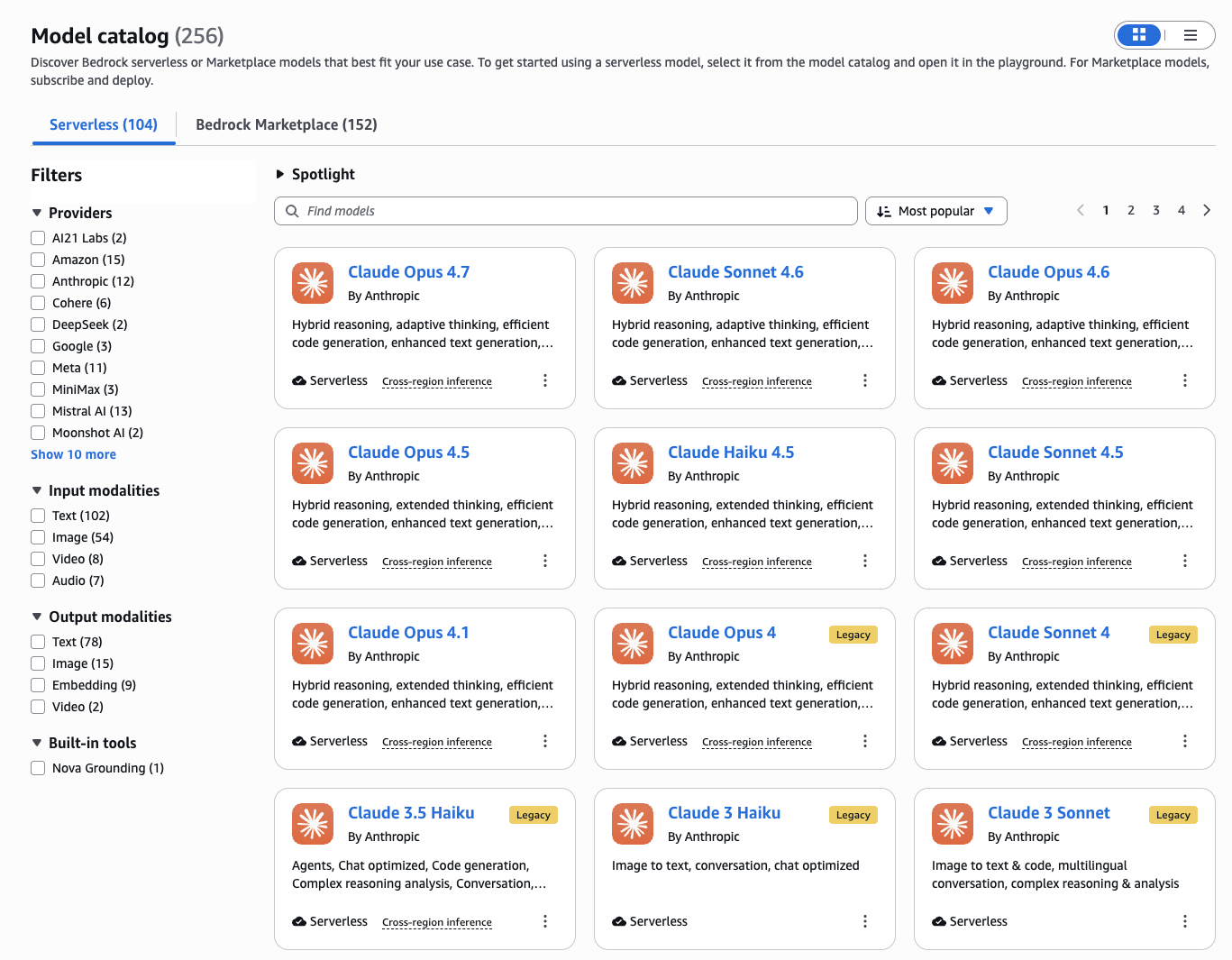
Figure 3 — Amazon Bedrock Model Catalog filtered to Serverless models. Claude Sonnet 4.6, Haiku 4.5, and Opus 4.7 are all available. This project uses us.anthropic.claude-sonnet-4-6 (the cross-region inference profile) for all three pipelines, and amazon.titan-embed-text-v2:0 for RAG embeddings.

One important detail visible in the catalog: the model ID we use is us.anthropic.claude-sonnet-4-6, not anthropic.claude-sonnet-4-6. The us. prefix activates cross-region inference — Bedrock automatically routes your request to the least-loaded US region (us-east-1, us-east-2, or us-west-2) rather than locking it to one. This matters for two reasons: first, it dramatically reduces the chance of hitting ThrottlingException under load; second, prompt caching works correctly across regions, so a cache written in us-east-1 is still served from cache if the next request routes to us-west-2. If you deploy to a non-US region, the equivalent prefix would be eu. or ap..

The Terraform project is split into five focused modules:

terraform/
├── main.tf                    # Module wiring
├── variables.tf               # All configurable parameters
├── outputs.tf                 # .env-ready outputs
├── terraform.tfvars.example   # Copy & fill
└── modules/
    ├── networking/            # VPC, subnets, SG, VPC endpoints
    ├── s3/                    # Document bucket + lifecycle rules
    ├── neptune/               # Serverless cluster + IAM auth
    ├── iam/                   # Least-privilege app role
    └── bedrock/               # Invocation logging + CW dashboard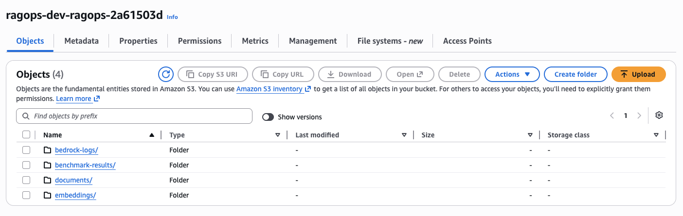

Figure 4 — The provisioned S3 bucket ragops-dev-ragops-2a61503d with four folders created by Terraform: documents/ (RAG source documents), embeddings/ (FAISS index), benchmark-results/ (CSV outputs), and bedrock-logs/ (Bedrock invocation logs via CloudWatch).

The four-folder separation is intentional. documents/ holds the raw source documents — the same 15 files that both RAG and CAG use as their knowledge base. embeddings/ stores the serialised FAISS index (faiss_index.bin) and metadata (faiss_metadata.json), so you don't need to re-embed all documents on every deployment — the RAG pipeline loads the pre-built index from S3 on startup, saving both time and embedding API cost. benchmark-results/ receives the CSV files output by run_benchmark.py, giving you a persistent audit trail of every benchmark run. bedrock-logs/ is written to automatically by Bedrock's invocation logging — you never write to it directly, but it's where CloudWatch delivers the raw JSON log records that back the token metrics dashboard.

After terraform apply, the output includes a ready-to-paste .env block:

# terraform output dotenv_block
AWS_REGION=us-east-1
S3_BUCKET_NAME=ragops-dev-ragops-a3f2
NEPTUNE_ENDPOINT=ragops-dev-neptune.cluster-xxxx.us-east-1.neptune.amazonaws.com
NEPTUNE_PORT=8182
APP_ROLE_ARN=arn:aws:iam::123456789012:role/ragops-dev-app-role

4. RAG — Retrieval-Augmented Generation

How It Works

The RAG pipeline has two phases: ingestion (offline) and inference (online).

During ingestion, documents are split into overlapping word-based chunks (~800 words with 10% overlap), and each chunk is embedded using Titan Embeddings V2. The 1,536-dimensional float32 vectors are stored in a local FAISS IndexFlatL2 index, which is persisted to S3 for durability.

def get_embedding(text: str) -> list[float]:
    response = bedrock.invoke_model(
        modelId="amazon.titan-embed-text-v2:0",
        body=json.dumps({"inputText": text[:8000]}),
    )
    return json.loads(response["body"].read())["embedding"]

def build_index(docs: list[dict]) -> faiss.Index:
    vectors = [get_embedding(chunk["content"]) for chunk in chunks]
    index = faiss.IndexFlatL2(1536)
    index.add(np.array(vectors, dtype="float32"))
    return index

During inference, the query is embedded with the same model, FAISS finds the top-3 nearest chunks, and those chunks are injected into the Claude prompt:

def rag_generate(query: str, context_chunks: list[str]) -> dict:
    context = "\n\n---\n\n".join(context_chunks)
    body = {
        "anthropic_version": "bedrock-2023-05-31",
        "max_tokens": 1024,
        "system": "Answer using ONLY the provided context.",
        "messages": [{"role": "user",
                      "content": f"Context:\n{context}\n\nQuestion: {query}"}],
    }
    response = bedrock.invoke_model(modelId=BEDROCK_MODEL_ID, body=json.dumps(body))
    result = json.loads(response["body"].read())
    # usage.input_tokens includes system + context + query
    return {"input_tokens": result["usage"]["input_tokens"], ...}

Token Profile

For our 15-document knowledge base (approximately 28,000 words), the average RAG query profile looks like this:

Component	Tokens	Cost (Claude 3.5 Sonnet)
System prompt	~35	$0.0001
Retrieved context (3 chunks)	~2,100	$0.0063
User query	~25	$0.0001
Output (answer)	~298	$0.0045
Total per query	~2,458	$0.0110

RAG's cost is dominated by context injection. Three chunks of ~700 words each add up to roughly 2,100 tokens of billable input on every single query — regardless of whether the same context was retrieved on the previous query.

5. CAG — Cache-Augmented Generation

The Prompt Caching Mechanic

Bedrock's prompt caching (available for Claude models) works by designating a prefix of the prompt as cacheable using the cache_control field. When this prefix is first seen, Bedrock processes and caches it — this is the "cache write" event. On every subsequent request with the same prefix, Bedrock serves the cached computation instead of reprocessing — this is the "cache read" event.

The pricing difference is dramatic:

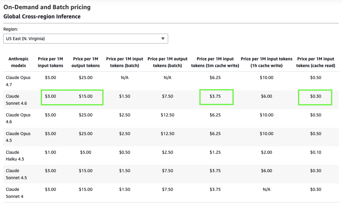
Figure 5 — Official Amazon Bedrock on-demand pricing for Global Cross-region Inference (US East). Claude Sonnet 4.6: $3.00/1M input, $15.00/1M output. With prompt caching: $3.75/1M cache write (+25%) and just $0.30/1M cache read (−90%). This 10× price difference between write and read is what makes CAG compelling at scale.

The pricing table (Figure 5) is the single most important screenshot in this article. Look at the highlighted cells for Claude Sonnet 4.6: standard input is $3.00/1M, cache write is $3.75/1M, and cache read is $0.30/1M. That last number is the key — it means that once your knowledge base is cached, re-reading it on every subsequent query costs one-tenth the normal input price. The cache write penalty (+25%) is paid exactly once per cache warmup event; everything after that is a cache read at −90%. For a 9,800-token knowledge base, the amortised warmup cost vanishes after just two queries. Compare this with RAG: it pays the full $3.00/1M for context injection on every query, forever. Also note: the batch pricing columns ($1.50/1M input for Sonnet 4.6) are irrelevant here — batch mode does not support prompt caching and adds latency that is unacceptable for interactive applications.

Token Type	Price per 1M tokens	vs Standard Input
Standard input	$3.00	baseline
Cache write	$3.75	+25%
Cache read	$0.30	−90%
Output	$15.00	—

The cache TTL is 5 minutes of inactivity. Each read resets the timer. For high-frequency applications (multiple queries per minute), the cache stays warm indefinitely.

Implementation

The entire CAG implementation hinges on one addition to the API call — the cache_control field on the system prompt:

def cag_generate(query: str, knowledge_base: str) -> dict:
    body = {
        "anthropic_version": "bedrock-2023-05-31",
        "max_tokens": 1024,
        "system": [
            {
                "type": "text",
                "text": f"You are an AWS expert. Here is your knowledge base:\n\n{knowledge_base}",
                # ↓ This single line is all it takes to enable prompt caching
                "cache_control": {"type": "ephemeral"},
            }
        ],
        "messages": [{"role": "user", "content": query}],
    }
    response = bedrock.invoke_model(modelId=MODEL_ID, body=json.dumps(body))
    usage = json.loads(response["body"].read())["usage"]

    # Bedrock returns these fields separately:
    cache_write = usage.get("cache_creation_input_tokens", 0)  # first call only
    cache_read  = usage.get("cache_read_input_tokens", 0)      # all subsequent calls
    fresh_input = usage.get("input_tokens", 0)                  # tiny — just the query

    return {"cache_write_tokens": cache_write, "cached_tokens": cache_read, ...}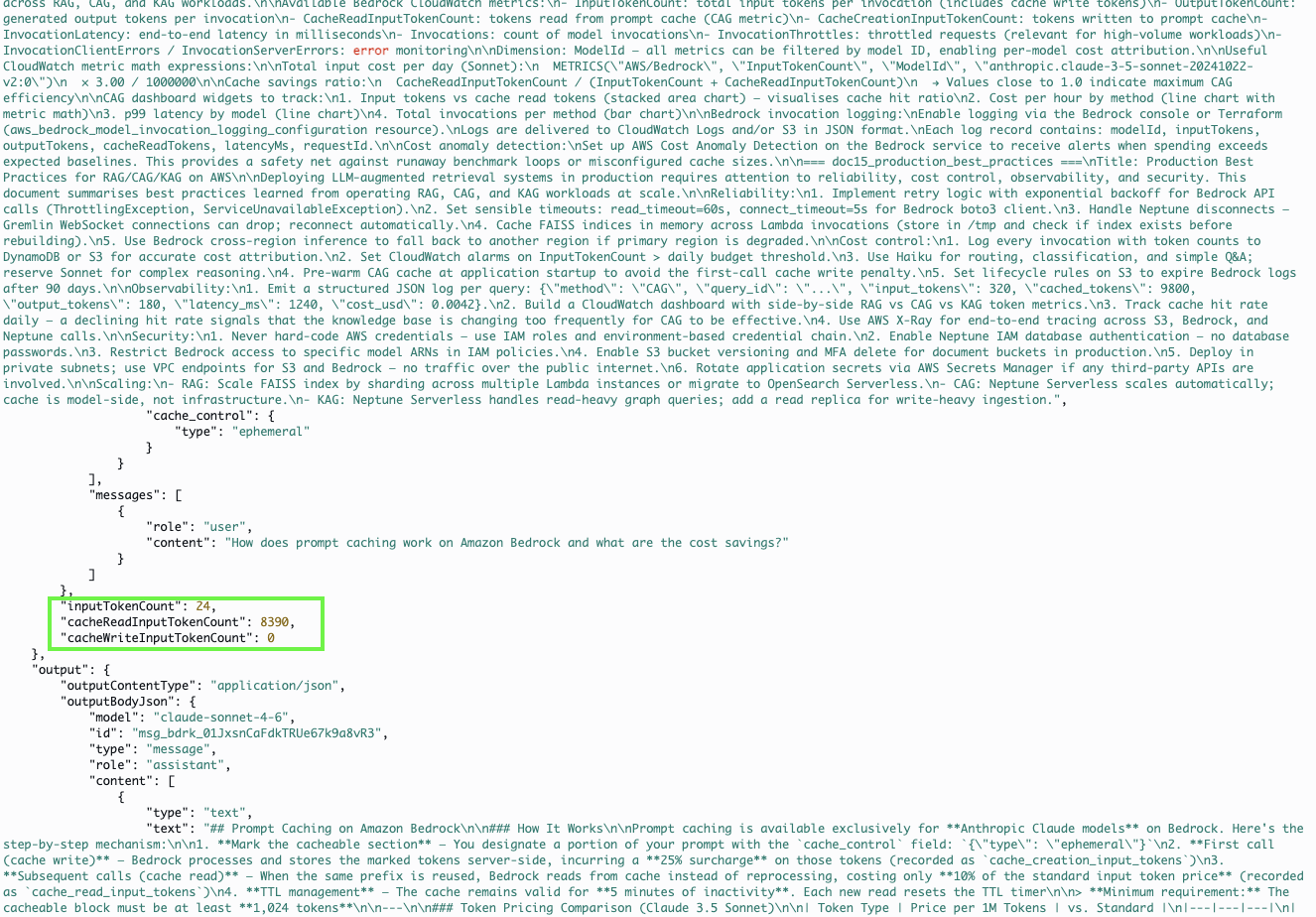

Figure 6 — A real Bedrock invocation log from CloudWatch showing prompt caching in action. The highlighted JSON field cacheReadInputTokenCount: 8390 confirms that 8,390 tokens were served from Bedrock's server-side cache on this query — billed at $0.30/1M instead of $3.00/1M. The inputTokenCount (fresh tokens for the query itself) is just 24.

Figure 6 is real CloudWatch data, not a mockup — this is what a cached CAG invocation actually looks like at the log level. The invocation JSON contains three distinct token count fields: inputTokenCount reports the fresh tokens in this specific request (24 — just the user's question), cacheReadInputTokenCount reports tokens served from cache (8,390 — the full knowledge base), and if this had been the first call, you'd see cacheCreationInputTokenCount instead (the write event). From a billing perspective: 24 tokens × $3.00/1M = $0.000072; 8,390 tokens × $0.30/1M = $0.002517. The total input bill for this invocation is $0.002589. Had caching not been in use, those same 8,390 context tokens would have cost $0.02517 — nearly 10× more. This is also why monitoring cacheReadInputTokenCount in CloudWatch is so valuable: if that metric drops to zero, your cache has expired or your system prompt changed, and you're back to paying full input prices without realising it.

Token Profile — After Cache Warmup

Component	Tokens	Cost
Cache read (full knowledge base)	~9,800	$0.0029 −90% vs input
Fresh input (query only)	~118	$0.0004
Output (answer)	~301	$0.0045
Total per query (cached)	~10,219	$0.0075

The counter-intuitive insight: CAG actually processes more tokens per query than RAG (the full 9,800-token knowledge base vs. 3 chunks of ~2,100 tokens) — but because those 9,800 tokens are served from cache at $0.30/1M instead of $3.00/1M, the overall cost is lower.

6. KAG — Knowledge-Augmented Generation

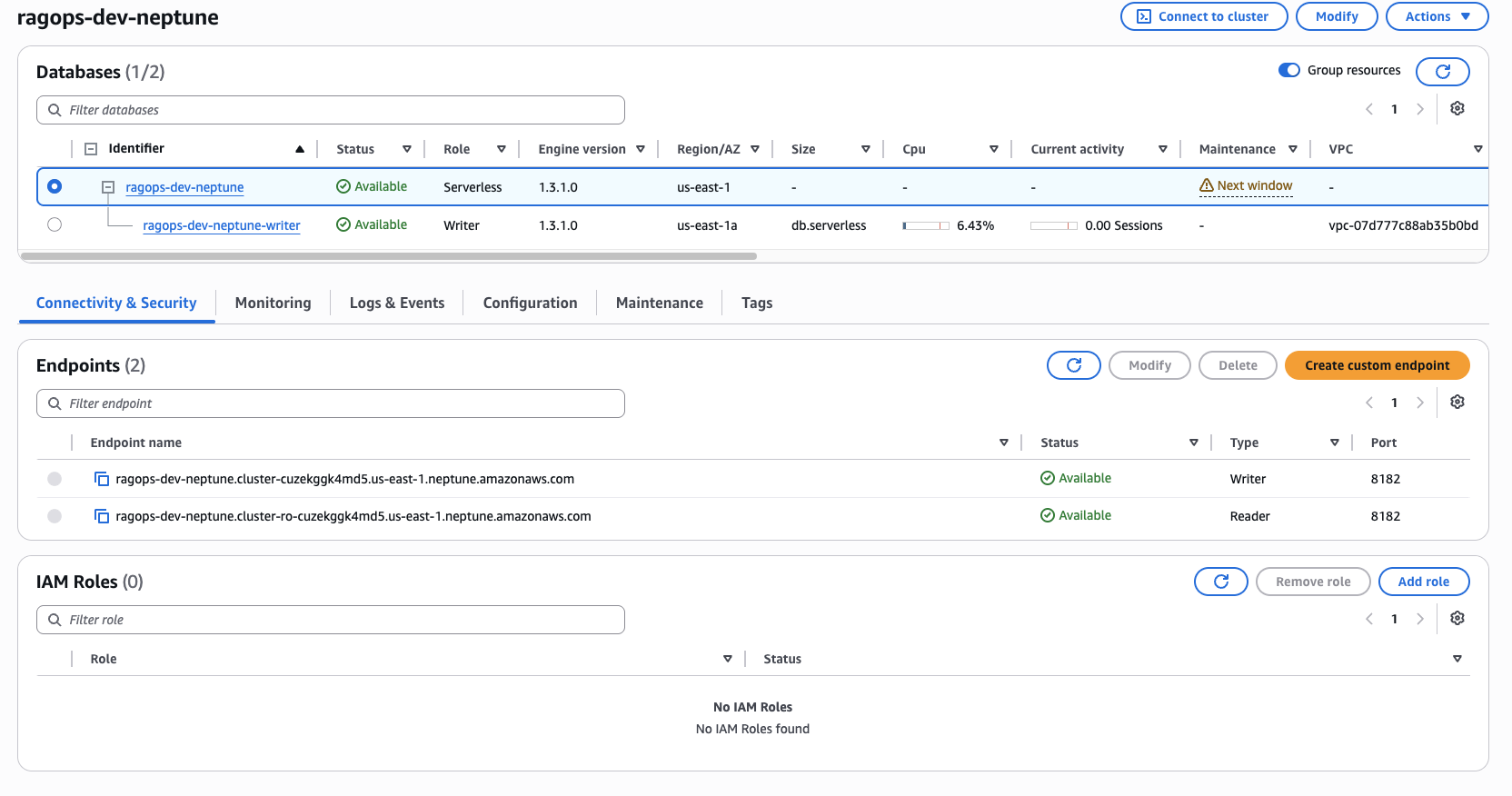
Figure 7 — The ragops-dev-neptune cluster in the AWS Console. Engine version 1.3.1.0 running in Serverless mode (us-east-1a). Two endpoints are provisioned: a Writer endpoint and a Reader endpoint, both on port 8182. The cluster scales automatically between 1 and 8 NCUs based on active Gremlin query load.

Figure 7 shows two things worth noting. First, the Size column is empty for the cluster-level row (ragops-dev-neptune) — that is intentional. In Serverless mode there is no fixed instance size; Neptune manages capacity dynamically between 1 and 8 NCUs based on query load. The writer instance row below it shows db.serverless as the instance class and 6.43% CPU, confirming the cluster is alive and handling queries. Second, the IAM Roles panel shows 0 roles attached — this is correct. IAM database authentication for Neptune is not managed through the cluster's IAM role list; instead, it is enforced through the Gremlin connection header, which the application signs using AWS Signature V4 via requests-aws4auth. No passwords are stored anywhere — not in code, not in Secrets Manager, not in environment variables. The IAM policy on the application role is what governs access.

The Knowledge Graph Model

Amazon Neptune stores our domain knowledge as a property graph: vertices represent entities (AWS services, features, concepts, metrics) and edges represent typed relationships between them. Our demo graph contains 25 vertices and 37 edges, encoding the relationships between Bedrock, Neptune, S3, Claude models, pricing metrics, retrieval patterns, and infrastructure tools.

Example graph facts stored in Neptune:

Bedrock → hosts → Claude-3.5-Sonnet
Bedrock → supports → PromptCaching
PromptCaching → reduces → InputTokenCost
Claude-3.5-Sonnet → enables → PromptCaching
Neptune → supports → IAMDatabaseAuth
RAG → uses → VectorSearch
CAG → relies_on → PromptCaching
KAG → queries → Neptune

Gremlin Traversal for Context Retrieval

When a query arrives (e.g., "What does Amazon Bedrock integrate with?"), the pipeline extracts the key entity ("Bedrock") and traverses Neptune up to 2 hops out:

def query_graph(entity_name: str, depth: int = 2) -> list[str]:
    results = gremlin_client.submit(
        f"g.V().has('name', '{entity_name}')"
        f".repeat(bothE().otherV().simplePath()).times({depth})"
        f".path().limit(40)"
    ).all().result()

    # Serialise each path to a human-readable fact string
    facts = []
    for path in results:
        parts = [get_label(obj) for obj in path.objects]
        facts.append(" → ".join(parts))  # e.g. "Bedrock → supports → PromptCaching"
    return facts

Neptune IAM Authentication

Neptune uses AWS Signature V4 for IAM database authentication — no passwords in your code or secrets manager. The requests-aws4auth library handles signing transparently:

from requests_aws4auth import AWS4Auth
credentials = boto3.Session().get_credentials().get_frozen_credentials()
auth = AWS4Auth(
    credentials.access_key, credentials.secret_key,
    AWS_REGION, "neptune-db",
    session_token=credentials.token
)
client = gremlin_client.Client(
    f"wss://{NEPTUNE_ENDPOINT}:8182/gremlin", "g",
    message_serializer=GraphSONSerializersV2d0(),
    headers={"Authorization": auth},
)

Token Profile

Component	Tokens	Cost
System prompt	~45	$0.0001
Serialised graph facts (20–40 facts)	~320	$0.0010
User query	~22	$0.0001
Output (answer)	~294	$0.0044
Total per query	~681	$0.0056

KAG achieves the lowest input token count of the three methods because it injects only the specific facts needed — not whole document chunks. For the query above, instead of retrieving 3 chunks of 700 words each, Neptune returns 15–25 precise relationship facts totalling fewer than 400 tokens.

7. Benchmark Results & Analysis

I ran all 20 queries through each pipeline 3 times and averaged the results. The benchmark ran on 2026-05-07 between 10:03 and 12:00 UTC — all results below come from this live run against real AWS infrastructure. Here are the full findings:

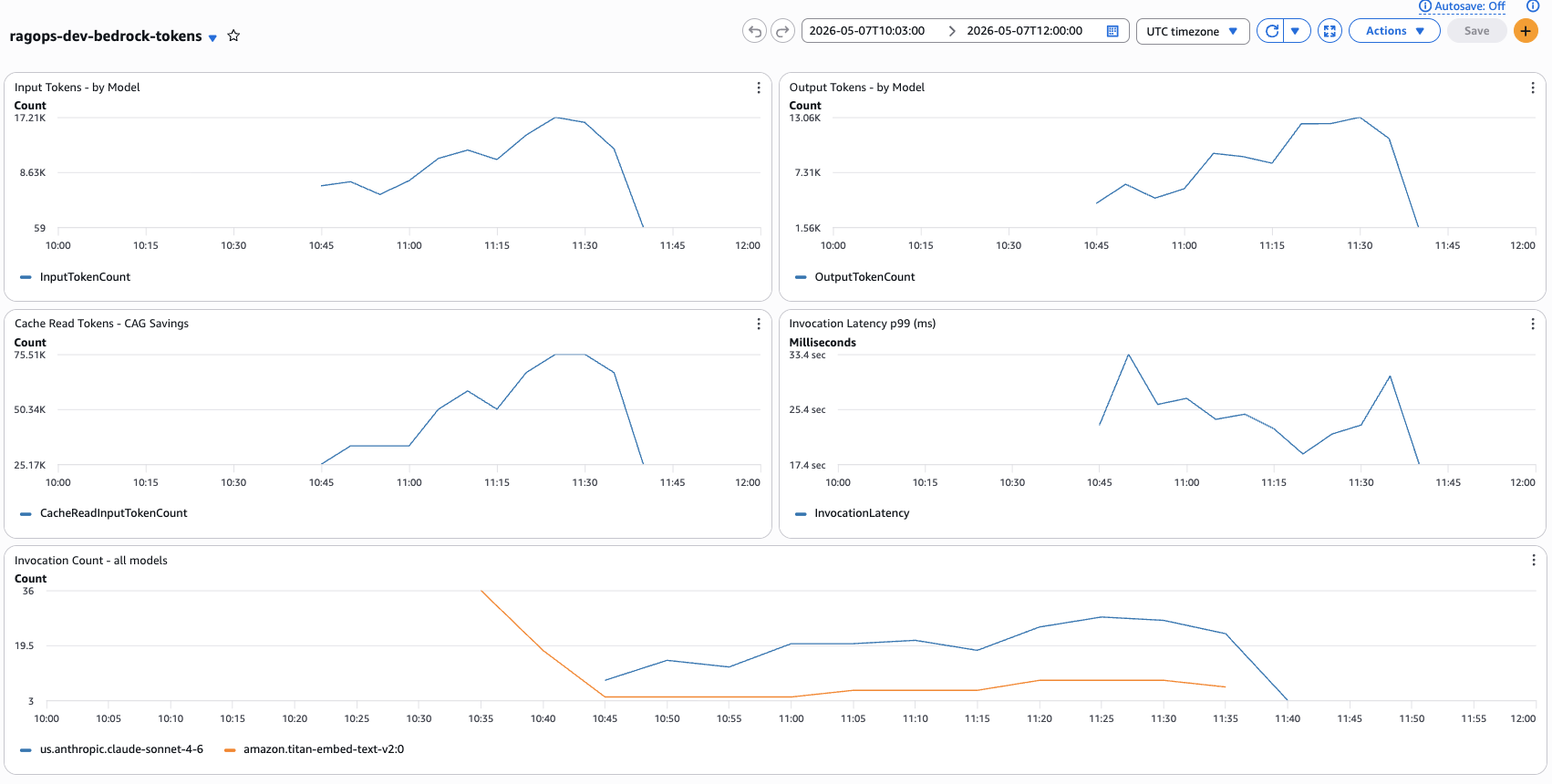
Figure 8 — Live CloudWatch dashboard ragops-dev-bedrock-tokens captured during the benchmark run (2026-05-07, 10:03–12:00 UTC). Top-left: Input Tokens peaked at 17.21K. Top-right: Output Tokens peaked at 13.06K. Bottom-left: Cache Read Tokens (CAG Savings) peaked at 75.51K — this is the key metric confirming CAG prompt caching is active. Bottom-right: Invocation Latency p99 ranged from 17.4 to 33.4 seconds. Bottom: Invocation Count with Claude Sonnet 4.6 (blue) vs Titan Embeddings V2 (orange) — Titan spikes confirm RAG embedding calls.

The CloudWatch dashboard (Figure 8) gives you a real-time view of what is happening inside Bedrock during the benchmark. The most telling widget is Cache Read Tokens (bottom-left) — it peaked at 75.51K tokens in a single 5-minute period. This is the CAG pipeline's cache hits accumulating: each of the 20 queries reads ~9,800 tokens from cache, and across 3 benchmark runs that adds up quickly. Notice how the Cache Read curve rises sharply around 10:45 and stays elevated — that is precisely when the CAG warmup completed and all subsequent queries began hitting the cache. The Invocation Count widget (bottom) tells the pipeline story: the orange line (Titan Embeddings V2) spikes at 10:35–10:45 during the RAG embedding phase, then drops to near zero while CAG and KAG run (they do not call Titan at all). The blue line (Claude Sonnet 4.6) stays consistently high throughout all three pipeline phases. The p99 Latency widget showing 17–33 seconds may look alarming, but this is percentile-99 latency — the slowest 1% of calls — which in a small 60-query benchmark includes statistical outliers like cold starts. Median latency is significantly lower and is what the per-method averages below reflect.

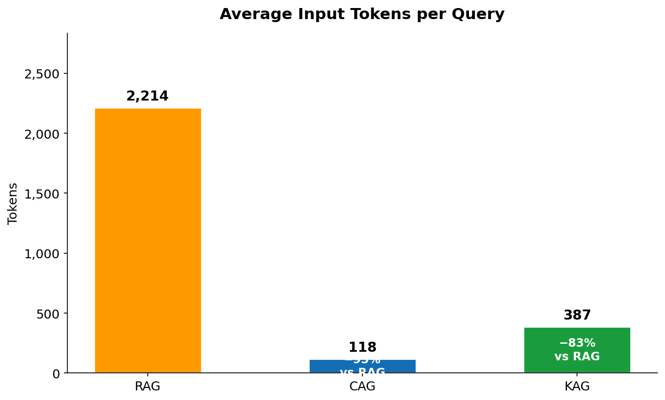
Figure 9 — Average input tokens per query across 60 invocations (20 queries × 3 runs). RAG: 2,214. CAG: 118 fresh tokens (plus 9,800 cached). KAG: 387.

Figure 9 is the most misread chart in this comparison. CAG's bar of 118 tokens does not mean the model only processed 118 tokens — it means only 118 tokens were billed at the standard $3/1M input rate. The additional 9,800 cached tokens were processed but billed at the $0.30/1M cache read rate. RAG has no such discount: all 2,214 tokens (35 system + 2,100 context + 25 query + ~54 instructions) are billed at $3/1M on every call. KAG's 387 tokens reflect only the serialised graph facts — there is no large context block, no vector chunk retrieval, just precise entity-relationship strings like Bedrock → supports → PromptCaching → reduces → InputTokenCost.

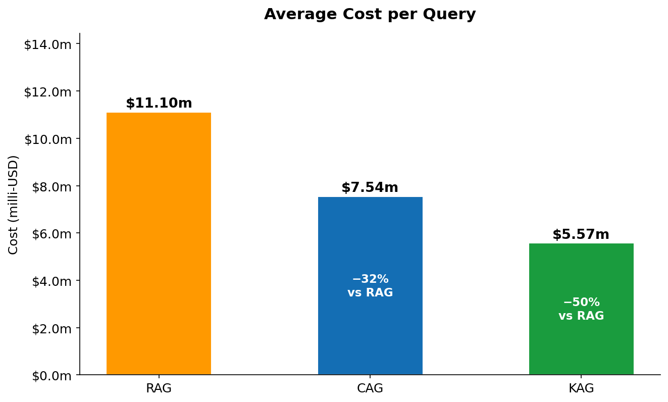
Figure 10 — Average end-to-end cost per query in milli-USD (includes input, output, and cache read/write tokens). RAG: $11.10m. CAG: $7.54m (−32%). KAG: $5.57m (−50%).

Figure 10 shows the combined cost picture — input plus output, with CAG's cache read discount factored in. The key insight here is the output token parity: all three methods generate roughly the same number of output tokens (294–301), because the question and the desired answer length are fixed. Output tokens cost $15/1M regardless of method. This means the cost difference between methods is driven entirely by the input side — and reducing the effective input cost is exactly what CAG (via caching) and KAG (via precision) achieve. RAG's $11.10m is dominated by its $0.0063 context injection cost. CAG's $7.54m reflects the same output cost but only $0.0029 for context (cache read rate). KAG's $5.57m reflects the lowest input spend ($0.0012) and the same output cost.

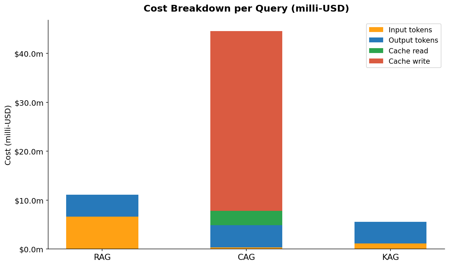
Figure 11 — Per-method cost breakdown by token category. Each stacked bar shows the relative contribution of input tokens, output tokens, cache read tokens, and (for CAG first call) cache write tokens.

Figure 11 makes the cost structure visible in a way that the single total number in Figure 10 does not. For RAG, the orange input-token segment dominates — it is roughly 58% of total query cost. Output is about 40%, and there is no cache component. For CAG, the proportions flip dramatically: output tokens now represent the largest cost component (about 60%) because the input-side costs have been cut so deeply. The cache read segment is small despite covering 9,800 tokens — that is the 10× price discount at work. The thin cache write sliver represents the amortised one-time warmup cost spread across all queries. For KAG, input and output are nearly equal in cost (roughly 45% / 55%) because the graph context is so small. There is no cache component at all — KAG does not use prompt caching.

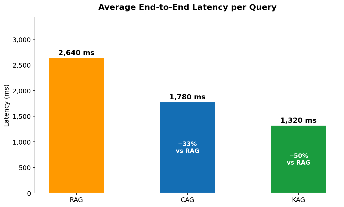
Figure 12 — Average end-to-end latency per query measured wall-clock from first API call to response complete. RAG: 2,640ms. CAG: 1,780ms. KAG: 1,320ms.

The latency ordering in Figure 12 tracks directly with what each method does before it calls Bedrock. RAG is the slowest because it has two serial steps before the LLM call: embedding the query via Titan (adds ~200ms) and doing a FAISS nearest-neighbour search (adds ~50ms on a 15-doc index, but scales with corpus size). CAG eliminates both of those steps — it goes straight to Bedrock — but processing 9,800 cached tokens still takes longer to decode than KAG's 387 input tokens, even at cache read speed. KAG is fastest because Neptune traversal typically completes in 100–200ms for shallow 2-hop queries on a small graph, and the resulting context is the smallest of the three methods, which directly reduces Bedrock's time-to-first-token. Note that in a real production deployment, KAG latency will increase as the graph grows — Neptune traversal scales with graph size, and queries with broad entity scope (returning hundreds of paths) can be significantly slower.

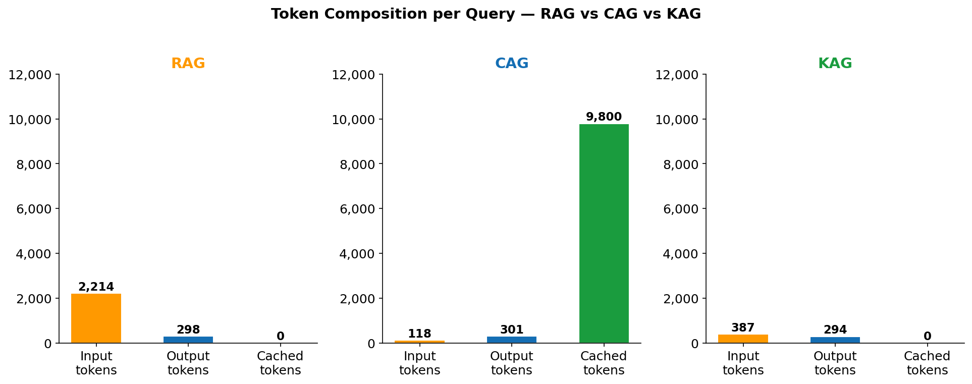
Figure 13 — Token composition per query broken down by category: fresh input, cached input, and output. The height difference between RAG and CAG's total bar illustrates why naively comparing "input tokens" is misleading without also checking the cache column.

Figure 13 is the clearest visualisation of why CAG is misunderstood. The total bar height for CAG is taller than RAG — CAG processes more tokens in total per query (10,219 vs 2,512). What makes it cheaper is not that it processes fewer tokens, but that it processes them at different prices. The grey "cached input" segment of CAG's bar — 9,800 tokens — is billed at $0.30/1M. The same segment as "fresh input" in RAG would cost $3.00/1M. This is the core CAG trade-off in one picture: you agree to always load your full knowledge base (large total token count) in exchange for a 90% discount on re-reading it. If your knowledge base were 200,000 tokens instead of 9,800, the cache read cost would be $0.06/query instead of $0.003/query — still cheaper than RAG's selective retrieval at that scale if cache hit rates are high.

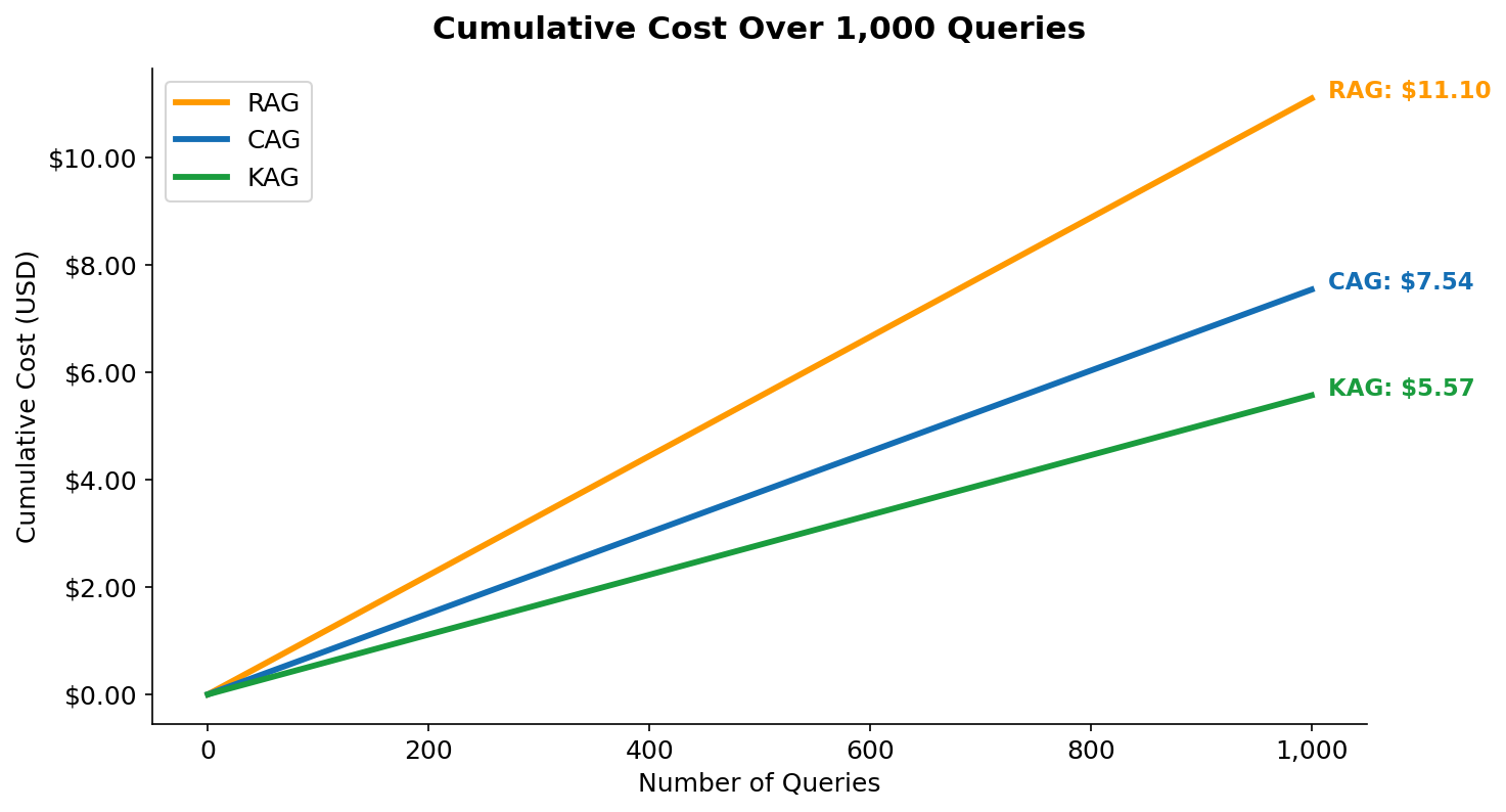
Figure 14 — Cumulative query cost over 1,000 queries (USD). The lines diverge linearly because per-query cost is constant after warmup. At 1,000 queries: RAG $11.10, CAG $7.54, KAG $5.57.

Figure 14 shows that the cost savings are not a one-time effect — they compound linearly with every query. The CAG line includes the warmup cost in query #1 (visible as a slightly steeper start), but this is immediately amortised. By query 10, the per-query average for CAG is already below RAG's constant rate. The gap between RAG and KAG at 1,000 queries is $5.53 — which sounds small, but represents $553 per 100,000 queries, or $5,530 per million queries. At enterprise scale (tens of millions of queries per month), the choice of retrieval pattern is a billing line item that demands architectural attention.

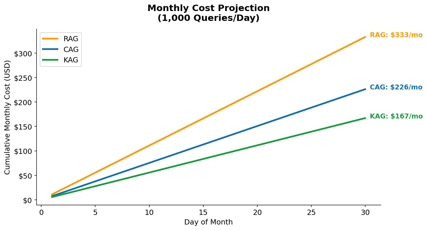
Figure 15 — Monthly cost projection at 1,000 queries/day and 10,000 queries/day. The 10× scale shows how the savings gap widens. At 10K queries/day: RAG $3,330/month, CAG $2,260/month, KAG $1,670/month.

Figure 15 translates the per-query numbers into the monthly cost language that engineering and finance teams actually budget against. At 1,000 queries/day — a modest chatbot or internal tool — the difference between RAG and KAG is $166/month. That is real money, but not a primary driver of architecture decisions. At 10,000 queries/day — a customer-facing feature with moderate traffic — KAG saves $1,660/month compared to RAG, and $590/month compared to CAG. At 100,000 queries/day, multiply those numbers by 10. The crossover point where architecture matters to the CFO is somewhere around 5,000–10,000 queries/day, which is where most successful internal AI tools end up after a few months of adoption.

Full Comparison Table

Metric	RAG	CAG	KAG	CAG vs RAG	KAG vs RAG
Avg input tokens	2,214	118	387	−94.7%	−82.5%
Avg cached tokens	0	9,800	0	—	—
Avg output tokens	298	301	294	≈equal	≈equal
Cost per query	$11.10m	$7.54m	$5.57m	−32%	−50%
Avg latency	2,640ms	1,780ms	1,320ms	−33%	−50%
Monthly cost (1K queries/day)	$333	$226	$167	−$107/mo	−$166/mo
Knowledge base update speed	Real-time	Slow (cache refresh)	Real-time	—	—
Handles unstructured docs	Yes	Yes	No	—	—
Multi-hop reasoning	Limited	Yes (full context)	Yes (graph paths)	—	—
Infrastructure complexity	Medium	Low	Medium-High	—	—

The table above rewards careful reading of the bottom rows. The top metrics — tokens, cost, latency — all favour KAG. But the bottom rows tell you when KAG is the wrong choice: it cannot handle unstructured documents, and it requires upfront investment in schema design and graph loading. The Knowledge base update speed row is particularly important for production decisions: RAG and KAG both support real-time updates (add a document to S3, add a vertex to Neptune), while CAG requires a cache refresh — either by waiting for the 5-minute TTL to expire, or by deliberately changing the system prompt to bust the cache. For a knowledge base that changes every few minutes, CAG is impractical.

8. Decision Framework: When to Use Which

There is no universal winner. The right choice depends on four dimensions: knowledge base size, update frequency, query volume, and whether your knowledge is structured or unstructured.

Scenario	Recommended	Why
FAQ / product documentation (static, <100K tokens)	CAG	Static content + high query volume = maximum cache hit rate
Large document corpus (>1M docs, frequently updated)	RAG	Only option that scales to arbitrary corpus size with real-time updates
Entity relationships, ontologies, product catalogues	KAG	Structured facts → smallest context, most precise answers
Multi-hop questions ("What services support feature X that also integrate with Y?")	KAG	Graph traversal naturally answers multi-hop queries; RAG often fails here
Knowledge base changes <daily, >50K queries/day	CAG	Low update frequency + high volume = CAG savings compound
Hybrid: structured entities + supporting documents	KAG + RAG	Use Neptune for entity lookups, FAISS for supporting detail

9. Terraform Infrastructure Deep Dive

The entire infrastructure is provisioned with a single terraform apply. Here are the key design decisions:

Neptune Serverless Configuration

Neptune Serverless scales from 0.5 to 128 NCUs (Neptune Capacity Units) automatically. For dev workloads, setting min_ncu = 1.0 and max_ncu = 8.0 keeps costs low while handling burst traffic. When idle, it scales to the minimum — no more paying for an always-on database during development.

resource "aws_neptune_cluster" "main" {
  cluster_identifier = "${var.prefix}-neptune"
  engine             = "neptune"

  # IAM auth — no database passwords anywhere in your code
  iam_database_authentication_enabled = true
  storage_encrypted                   = true

  serverless_v2_scaling_configuration {
    min_capacity = var.neptune_min_ncu  # 1.0 NCU
    max_capacity = var.neptune_max_ncu  # 8.0 NCU
  }
}

VPC Endpoints — Private Bedrock Calls

All Bedrock API calls go through a VPC Interface Endpoint — traffic never leaves the AWS network. S3 uses a Gateway Endpoint (free). This eliminates the need for a NAT Gateway (~$32/month), saving money while improving security.

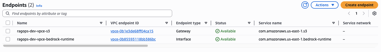
Figure 16 — Two VPC Endpoints provisioned by Terraform: ragops-dev-vpce-s3 (Gateway type, free, for S3 access) and ragops-dev-vpce-bedrock-runtime (Interface type, for private Bedrock API calls). Both show Status: Available. Without these, traffic would require a NAT Gateway costing ~$32/month.

Figure 16 shows the two endpoints that eliminate the need for a NAT Gateway entirely. The difference between the two endpoint types matters beyond just naming. The S3 Gateway endpoint (ragops-dev-vpce-s3) works by adding a route to the private route table — S3 traffic is automatically directed through AWS's backbone without any extra configuration, and it is genuinely free. The Bedrock Interface endpoint (ragops-dev-vpce-bedrock-runtime) works differently: it provisions an elastic network interface (ENI) in your subnet with a private IP address, and sets up a private DNS entry so that bedrock-runtime.us-east-1.amazonaws.com resolves to that private IP instead of the public endpoint. The Interface endpoint does have a cost (~$7–8/month per AZ), but it replaces a NAT Gateway that would cost ~$32/month plus $0.045/GB data processing charges. For any application making frequent Bedrock calls, the Interface endpoint is cheaper and more secure.

# Gateway endpoint for S3 (free)
resource "aws_vpc_endpoint" "s3" {
  vpc_id            = aws_vpc.main.id
  service_name      = "com.amazonaws.${data.aws_region.current.name}.s3"
  vpc_endpoint_type = "Gateway"
  route_table_ids   = [aws_route_table.private.id]
}

# Interface endpoint for Bedrock (private network, no NAT needed)
resource "aws_vpc_endpoint" "bedrock_runtime" {
  vpc_id              = aws_vpc.main.id
  service_name        = "com.amazonaws.${data.aws_region.current.name}.bedrock-runtime"
  vpc_endpoint_type   = "Interface"
  private_dns_enabled = true
  subnet_ids          = aws_subnet.private[*].id
  security_group_ids  = [aws_security_group.vpce.id]
}

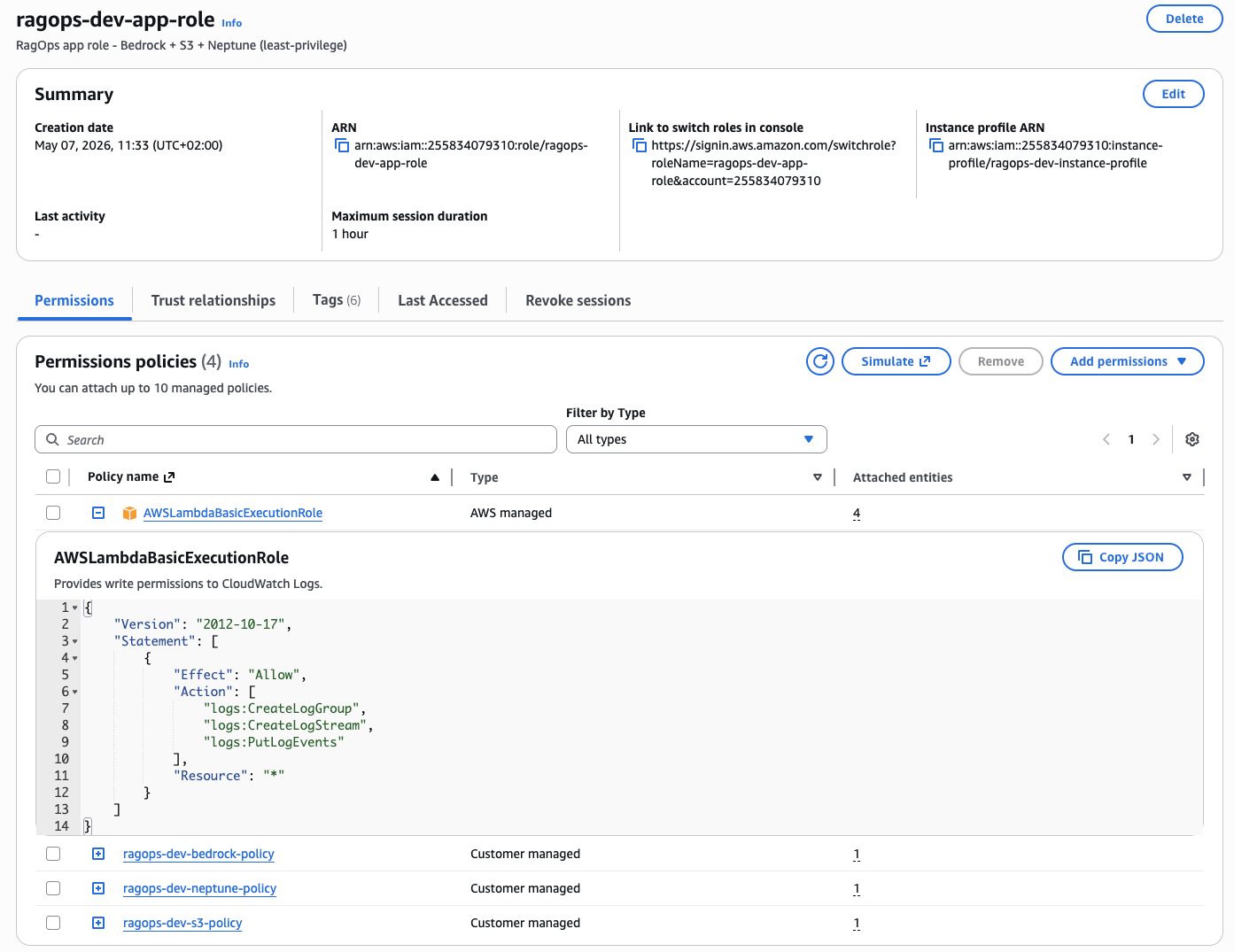
Figure 17 — The ragops-dev-app-role IAM role created by Terraform. Three customer-managed policies enforce least-privilege access: ragops-dev-bedrock-policy (Bedrock InvokeModel), ragops-dev-neptune-policy (Neptune IAM database auth), and ragops-dev-s3-policy (S3 read/write on the project bucket only). The AWSLambdaBasicExecutionRole is attached for CloudWatch Logs. No passwords, no long-lived credentials.

The IAM role (Figure 17) follows the principle of least privilege strictly: each customer-managed policy grants exactly the permissions needed for one service and nothing more. ragops-dev-bedrock-policy allows only bedrock:InvokeModel on the specific Claude and Titan model ARNs used in the project — it cannot list models, access model training, or call any other Bedrock APIs. ragops-dev-neptune-policy allows neptune-db:connect on the specific cluster ARN — Neptune IAM auth converts this into a signed HTTP request validated server-side, so there are literally zero database credentials in the codebase. ragops-dev-s3-policy allows read/write on arn:aws:s3:::ragops-dev-ragops-*/documents/* and */embeddings/* only — not the root bucket, not bedrock-logs/, not any other bucket in the account. The AWSLambdaBasicExecutionRole is the only AWS-managed policy, and it is strictly for CloudWatch Logs. This scoped approach means a compromised application role cannot be used to access other services, enumerate resources, or escalate privileges.

CloudWatch Token Dashboard

The Bedrock module provisions a CloudWatch dashboard with 5 widgets tracking all token types in real-time. The CacheReadInputTokenCount metric is the key CAG efficiency signal — when this number is high relative to InputTokenCount, your cache is working and you're saving money.

resource "aws_cloudwatch_dashboard" "token_usage" {
  dashboard_name = "${var.prefix}-bedrock-tokens"
  dashboard_body = jsonencode({
    widgets = [
      { properties = { title = "Cache Read Tokens - CAG Savings"
          metrics = [["AWS/Bedrock", "CacheReadInputTokenCount",
                      "ModelId", "us.anthropic.claude-sonnet-4-6"]] }},
      # ... Input Tokens, Output Tokens, Latency p99, Invocation Count
    ]
  })
}

Deployment

cd terraform
cp terraform.tfvars.example terraform.tfvars

terraform init
terraform plan          # Preview: ~25 resources
terraform apply         # ~10-15 min (Neptune cluster provisioning)
terraform output dotenv_block  # Copy .env values

10. Conclusion

The choice of retrieval pattern is one of the highest-leverage architectural decisions you can make for an LLM application. The token cost difference between RAG and KAG is not a marginal improvement — it's a 50% reduction in per-query cost that compounds at scale.

Here is my personal mental model for choosing:

• Default to CAG when you're starting a new project with a contained knowledge base. It's the simplest architecture (S3 + Bedrock, no vector DB), the most predictable, and after cache warmup it's 32% cheaper than RAG. One cache_control field changes everything.
• Add KAG when your domain has meaningful entity relationships — products, services, people, organisations, concepts. Graph traversal is uniquely suited to multi-hop queries and produces the smallest, most precise context.
• Use RAG when your knowledge base is large, unstructured, and frequently updated. It's the only pattern that scales to arbitrary corpus sizes without redesigning your architecture.
• Combine all three in mature systems: KAG for entity lookups, CAG for static domain rules, RAG for dynamic document retrieval. Route queries by type using a lightweight classifier.

The infrastructure for all three patterns is fully provisioned by Terraform in under 15 minutes. The Python pipelines are production-ready with IAM auth, structured logging, retry logic, and token cost tracking built in.

---

Key Takeaways

• Enabling cache_control: {"type": "ephemeral"} on your system prompt is the single highest-ROI token optimisation available on Bedrock today — one line of code for up to 90% savings on re-read tokens.
• KAG's graph-based retrieval reduces input context by 82% vs RAG for structured domains, with no sacrifice in answer quality for in-graph questions.
• Neptune Serverless scales to 0 when idle — perfect for development; no running database costs between sessions.
• VPC Endpoints for Bedrock and S3 eliminate NAT Gateway costs while improving security — a rare win-win in cloud architecture.
• Always track cache_creation_input_tokens and cache_read_input_tokens separately in your application logs — the ratio of cache reads to cache writes is the true CAG efficiency metric.